1. 선형회귀
선형회귀는 종속변수와 독립변수간의 선형 관계를 모델링하는 방법이다.
주로 예측, 상관분석, 추정하는 문제에 사용한다.
선형회귀 모델링의 결과는 하나의 직선이다.
직선의 주요 특성은 Coefficient(가중치), Intercept(절편)이다.
여기서 가중치는 기울기를 의미한다.
만약 데이터에 비선형적인 관계나 이상치가 많은 경우엔 다른 회귀 모델을 사용해야 한다.
2. Rent 데이터셋
선형회귀를 이해하고 사용하기 위한 예시로 Rent 데이터셋을 사용한다.
Rent는 집 렌트에 관련된 데이터셋이다.
import numpy as np
import pandas as pd
import seaborn as sns

rent_df = pd.read_csv('/content/drive/MyDrive/KDT/머신러닝과 딥러닝/data/rent.csv')
read_csv를 사용하여 csv파일을 연다.
# 데이터 정보
rent_df.info()
output>>
<class 'pandas.core.frame.DataFrame'>
RangeIndex: 4746 entries, 0 to 4745
Data columns (total 12 columns):
 #   Column             Non-Null Count  Dtype
---  ------             --------------  -----
 0   Posted On          4746 non-null   object
 1   BHK                4743 non-null   float64
 2   Rent               4746 non-null   int64
 3   Size               4741 non-null   float64
 4   Floor              4746 non-null   object
 5   Area Type          4746 non-null   object
 6   Area Locality      4746 non-null   object
 7   City               4746 non-null   object
 8   Furnishing Status  4746 non-null   object
 9   Tenant Preferred   4746 non-null   object
 10  Bathroom           4746 non-null   int64
 11  Point of Contact   4746 non-null   object
dtypes: float64(2), int64(2), object(8)
memory usage: 445.1+ KB
info()를 통해 데이터를 살펴보면
BHK, Size외에는 모두 non-null이다.
BHK, Rent, Size, Bathroom을 제외하곤 모두 문자열이다.
각각 항목의 의미는
- Posted On: 매물 등록 날짜
- BHK: 베드, 홀, 키친의 개수
- Rent: 렌트비
- Size: 집 크기
- Floor: 총 층수 중 몇층
- Area Type: 공용공간을 포함하는지, 집의 면적만 포함하는지
- Area Locality: 지역
- City: 도시
- Furnishing Status: 풀옵션 여부
- Tenant Preferred: 선호하는 가족형태
- Bathroom: 화장실 개수
- Point of Contact: 연락할 곳
통계적인 데이터 요약을 보기 위해선 describe() 메서드를 사용한다.
decribe()는 주로 이상치를 확인하기 위해 사용한다. 현재 수치데이터는 위 4개 뿐이므로 4개의 column 정보만 출력된다.
# 수치 정보
round(rent_df.describe(), 2)
output>>
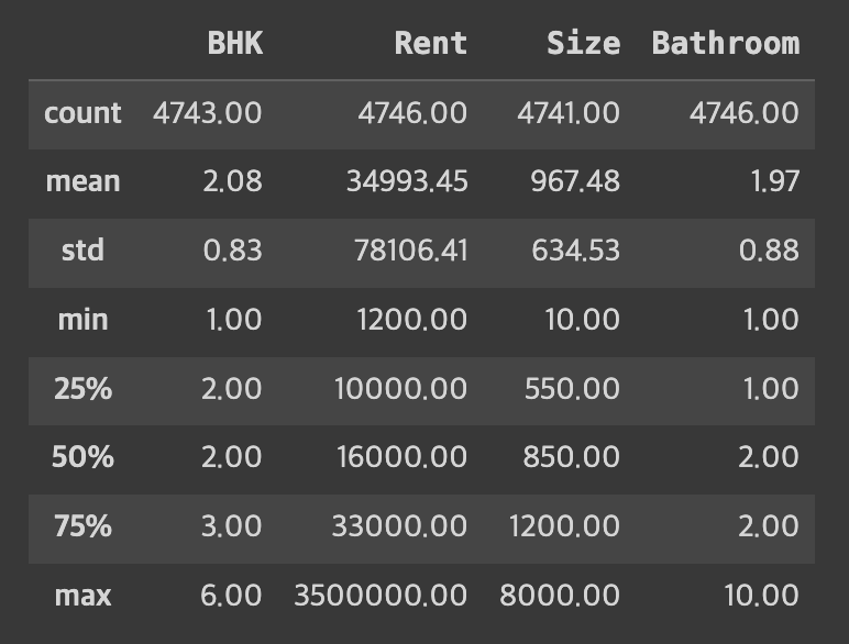
Rent 비용의 최대값이 많이 높이보인다. 이상치로 판단할지는 더 알아봐야할 것 같다.
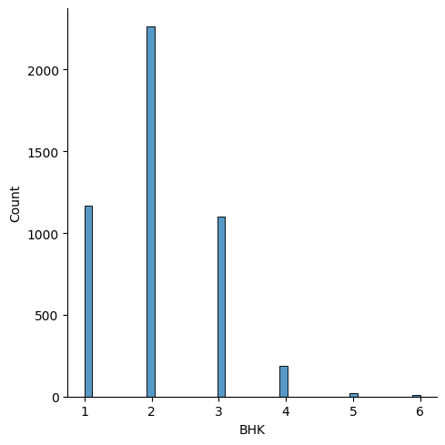
2-1. plot
다음으로 데이터들을 시각적으로 확인하기 위해 displot()을 사용해보자.
# 관계 시각화
sns.displot(rent_df['BHK'])
output>>
# 관계 시각화
sns.displot(rent_df['Rent'])
output>>
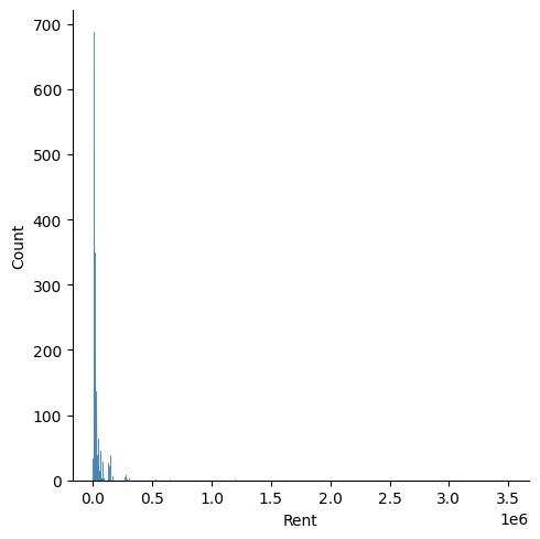
Rent의 경우 데이터는 0.0~0.5에 밀집되어 있는 것으로 보여지지만 x축이 3.5까지 펼쳐져 있는 것을 볼 수 있다.
x축의 범위가 괜히 이런 것이 아니다. 3.5까지 데이터가 존재하기 때문에 펼쳐진 것이다.
앞서 본 Rent 3500000.00 값이 그 원인인 것 같다.
# 데이터 정렬
rent_df['Rent'].sort_values()
output>>
4076       1200
285        1500
471        1800
2475       2000
146        2200
         ...
1459     700000
1329     850000
827     1000000
1001    1200000
1837    3500000
Name: Rent, Length: 4746, dtype: int64
최대값과 그 다음 값으 차이가 생각보다 많지 않은걸 보니 이상치는 아닌 것 같다.
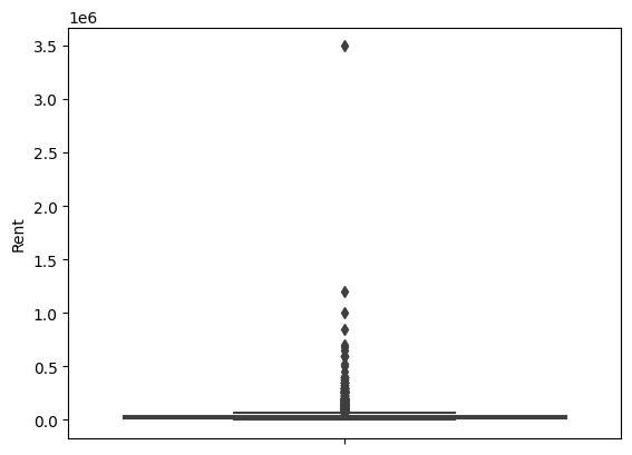
이상치를 확인하기 가장 좋은 그래프는 boxplot이다. 확실하게 확인해보자.
sns.boxplot(y=rent_df['Rent'])output>>
sns.boxplot(y=rent_df['BHK'])output>>
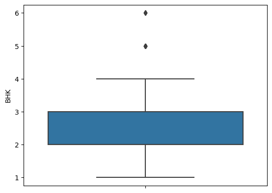
Rent의 경우 괘나 동떨어진 데이터가 존재하지만 분포가 충분히 연속적이라면 이상치로 보지 않기도 하기 때문에 그냥 넘어가도록 하자.
2-2. 데이터 전처리
na값이 있는 row아예 지우거나 중앙값 혹은 평균값으로 대체하는 과정이다.
# 결측치
rent_df.isna().sum()
output>>
Posted On            0
BHK                  3
Rent                 0
Size                 5
Floor                0
Area Type            0
Area Locality        0
City                 0
Furnishing Status    0
Tenant Preferred     0
Bathroom             0
Point of Contact     0
dtype: int64
na값들이 중앙값으로 대체되어도 큰 문제가 되지 않는다고 가정하고 진행한다.
# 중앙값
rent_df.median()
output>>
BHK             2.0
Rent        16000.0
Size          850.0
Bathroom        2.0
dtype: float64
숫자형 데이터들의 중앙값만을 반환함.
rent_df = rent_df.fillna(rent_df.median())
rent_df.isna().mean()
output>>
Posted On            0.0
BHK                  0.0
Rent                 0.0
Size                 0.0
Floor                0.0
Area Type            0.0
Area Locality        0.0
City                 0.0
Furnishing Status    0.0
Tenant Preferred     0.0
Bathroom             0.0
Point of Contact     0.0
dtype: float64
이제 결측치는 모두 처리하였다.
# 데이터 정보
rent_df.info()
output>>
<class 'pandas.core.frame.DataFrame'>
RangeIndex: 4746 entries, 0 to 4745
Data columns (total 12 columns):
 #   Column             Non-Null Count  Dtype
---  ------             --------------  -----
 0   Posted On          4746 non-null   object
 1   BHK                4746 non-null   float64
 2   Rent               4746 non-null   int64
 3   Size               4746 non-null   float64
 4   Floor              4746 non-null   object
 5   Area Type          4746 non-null   object
 6   Area Locality      4746 non-null   object
 7   City               4746 non-null   object
 8   Furnishing Status  4746 non-null   object
 9   Tenant Preferred   4746 non-null   object
 10  Bathroom           4746 non-null   int64
 11  Point of Contact   4746 non-null   object
dtypes: float64(2), int64(2), object(8)
memory usage: 445.1+ KB
2-3. 라벨 인코딩
나머지 문자열 데이터들을 라벨 인코딩 처리를 한다.
라벨 인코딩을 하는데 변환해야하는 라벨의 종류가 매우 많으면 곤란하므로 unique()와 nunique()를 통해 종류와 개수를 확인한다,
# 유니크한 종류의 개수
# Floor, Area Type, Area Locality, City, Furnishing Status, Tenant Preferred, Point of Contact
li = ['Floor', 'Area Type', 'Area Locality', 'City', 'Furnishing Status', 'Tenant Preferred', 'Point of Contact']
uni = 0
for i in li:
    print(i, rent_df[i].nunique())
output>>
Floor 480
Area Type 3
Area Locality 2235
City 6
Furnishing Status 3
Tenant Preferred 3
Point of Contact 3
종류가 너무 많으면 라벨 인코딩하기 쉽지 않다. 데이터를 확인하고 범위를 구분하여 라벨링을 할 수도 있지만 지금은 넘어가도록 한다.
Area Type, City, Furnishing Status을 제외한 column은 제거하여 데이터를 정리해보자.
rent_df.drop(['Floor', 'Area Locality', 'Tenant Preferred', 'Point of Contact', 'Posted On'], axis=1, inplace=True)
rent_df.info()
output>>
<class 'pandas.core.frame.DataFrame'>
RangeIndex: 4746 entries, 0 to 4745
Data columns (total 7 columns):
 #   Column             Non-Null Count  Dtype
---  ------             --------------  -----
 0   BHK                4746 non-null   float64
 1   Rent               4746 non-null   int64
 2   Size               4746 non-null   float64
 3   Area Type          4746 non-null   object
 4   City               4746 non-null   object
 5   Furnishing Status  4746 non-null   object
 6   Bathroom           4746 non-null   int64
dtypes: float64(2), int64(2), object(3)
memory usage: 259.7+ KB
남은 문자열 데이터를 바로 One Hot Encoding하여 숫자화를 한다.
rent_df = pd.get_dummies(rent_df, columns=['Area Type', 'City', 'Furnishing Status'])
rent_df.info()
output>>
<class 'pandas.core.frame.DataFrame'>
RangeIndex: 4746 entries, 0 to 4745
Data columns (total 16 columns):
 #   Column                            Non-Null Count  Dtype
---  ------                            --------------  -----
 0   BHK                               4746 non-null   float64
 1   Rent                              4746 non-null   int64
 2   Size                              4746 non-null   float64
 3   Bathroom                          4746 non-null   int64
 4   Area Type_Built Area              4746 non-null   uint8
 5   Area Type_Carpet Area             4746 non-null   uint8
 6   Area Type_Super Area              4746 non-null   uint8
 7   City_Bangalore                    4746 non-null   uint8
 8   City_Chennai                      4746 non-null   uint8
 9   City_Delhi                        4746 non-null   uint8
 10  City_Hyderabad                    4746 non-null   uint8
 11  City_Kolkata                      4746 non-null   uint8
 12  City_Mumbai                       4746 non-null   uint8
 13  Furnishing Status_Furnished       4746 non-null   uint8
 14  Furnishing Status_Semi-Furnished  4746 non-null   uint8
 15  Furnishing Status_Unfurnished     4746 non-null   uint8
dtypes: float64(2), int64(2), uint8(12)
memory usage: 204.1 KB
이처럼 라벨링을 하지 않고 One Hot Encoding을 할 수 있다.
이제 학습을 위해 독립변수와 종속변수를 나누고 train_test_split()을 사용하여 데이터를 섞어보자.
from sklearn.model_selection import train_test_split

X = rent_df.drop('Rent', axis=1) # 독립변수
y = rent_df['Rent'] # 종속변수

X_train, X_test, y_train, y_test = train_test_split(X, y, test_size=0.2, random_state=10)
test 개수
X_test.shape, y_test.shapeoutput>>
((950, 15), (950,))3. 선형 회귀(Linear Regression)
from sklearn.linear_model import LinearRegression

lr = LinearRegression()

lr.fit(X_train, y_train)

pred = lr.predict(X_test)

print(pred)
output>>
[ 1.85666954e+05  6.56319414e+04  3.79216873e+04  4.07492370e+04
  1.53644199e+04  1.03007898e+04  3.18519243e+04 -1.02863484e+03
  3.54652859e+03  5.49046889e+04  5.54039274e+04  1.24942586e+04
 -7.15496087e+03 -2.24552215e+04  9.53769064e+04  2.25665611e+03
  1.45745486e+04  4.21565876e+04  1.52484012e+04 -5.81255961e+01
  1.82136631e+03 -3.71785273e+03 -2.53960269e+04 -2.31902805e+04
  7.37835272e+04  4.71180750e+04  3.63188490e+03  4.32519136e+04
  4.55754646e+04  1.67146596e+04  7.78473203e+04 -1.24128261e+04
...
  4.55332198e+04 -1.84494572e+04 -1.33752336e+03 -1.10155016e+04
  1.11303737e+05  4.90287907e+04  2.73333152e+04  2.19765910e+04
  3.18821922e+04  7.13294239e+04 -7.06638250e+01 -5.89492961e+03
 -1.53683901e+04  1.12435924e+05  1.70856553e+04  8.86286828e+04
  8.22742616e+04  1.45745486e+04  5.03139001e+04  5.25984290e+04
  1.72155125e+04  1.52729424e+04]
총 950개의 예측 결과이다. 데이터 총 개수인 4746의 20%에 해당한다.
예측 결과만 봐서는 제대로 예측했는지 알 수 없다.
선형 회귀 모델은 MSE, MAE, RMSE의 평가 지표를 사용하여 성능을 비교한다.
4. 평가 지표
2023.12.25 - [분류 전체보기] - [머신러닝] MSE, MAE, RMSE
[머신러닝] MSE, MAE, RMSE
평가지표 선형회귀 모델의 성능을 평가하고 비교하기 위해 사용되는 평가지표. 평가지표 예시에 사용될 값. p = np.array([3, 4, 5]) # 예측값 act = np.array([1, 2, 3]) # 실제값 MSE(Mean Squared Error) 예측값과
caramelbottle.tistory.com
5. 평가 지표 적용하기
from sklearn.metrics import mean_absolute_error, mean_squared_error
지표의 연산 결과가 작을수록 성능이 좋다고 볼 수 있다.
5-1. MSE
mean_squared_error(y_test, pred)output>>
1717185779.00210675-2. MAE
mean_absolute_error(y_test, pred)output>>
22779.177225438945-3. RMSE
mean_squared_error(y_test, pred, squared=False)output>>
41438.9403701652
각 지표는 절대적인 값이지만 결과끼리 비교해야 의미가 있다.
데이터를 조금 변경하여 오차를 줄이는 작업을 해보자.
X_train.drop(1837, inplace=True)

y_train.drop(1837, inplace=True)
이전에 이상치로 의심했던 Rent의 최대값 row를 제거한 후에 다시 RMSE를 구해본다.
lr.fit(X_train, y_train)

mean_squared_error(y_test, pred, squared=False)
output>>
41377.570302348391837 삭제 전: 41438.9403701652
1837 삭제 후: 41377.57030234839
약간이지만 성능이 좋아진 것을 볼 수 있다.
6. 결론
선형회귀는 예측을 위해 사용한다.
평가지표는 상황에 따라 골라서 사용한다.
이상치는 되도록 제거하는 것이 성능에 좋다.
'AI > 머신러닝 - 예제' 카테고리의 다른 글
| [머신러닝 - 예제] 손글씨 데이터셋 - 서포트 벡터머신(SVM) (0) | 2023.12.28 |
|---|---|
| [머신러닝 - 예제] Human Resource 데이터셋 - 로지스틱 회귀 (0) | 2023.12.27 |
| [머신러닝 - 예제] Bike 데이터셋 - 의사 결정 나무 (1) | 2023.12.26 |
| [머신러닝 - 예제] 타이타닉 데이터셋 - 캐글 데이터셋 (0) | 2023.12.25 |
| [머신러닝 - 예제] 아이리스 데이터셋 - 사이킷런 데이터셋 (1) | 2023.12.22 |

댓글